Wafer Probe Test (Wafer Sort): Bin Maps, Probe Marks and Defect Correlation
Averroes
Nov 10, 2026
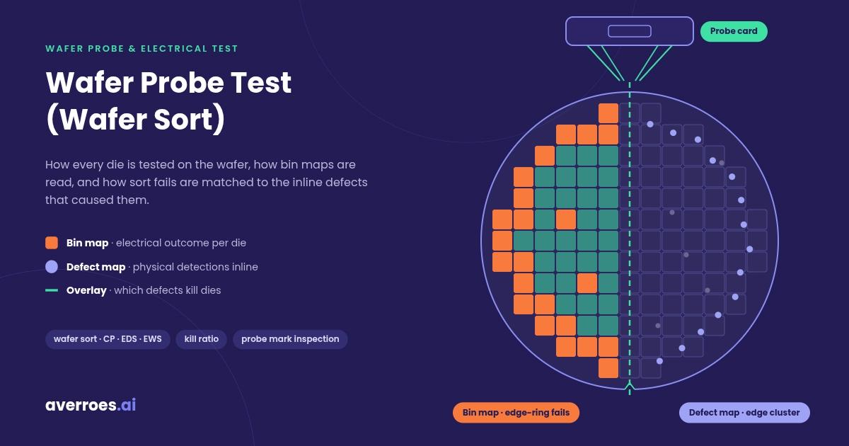
A wafer probe test, also called wafer sort or circuit probe, is the electrical test of every die on a finished wafer before it is diced. A prober aligns the wafer, a probe card touches each die’s pads, and a tester runs parametric and functional tests. Each die gets a bin code, and the result is a wafer bin map. Overlaying that bin map on inline defect maps shows which visual defects actually kill dies.
Wafer probe test is Stage 05 of the semiconductor manufacturing process, between front-end fabrication and assembly. This guide from Averroes.ai, an AI visual inspection platform for manufacturers, covers how the test runs, how to read its bin maps, how probe marks are inspected, and how sort results are correlated with inline defect data.
Key Notes
Wafer probe test goes by several names: wafer sort, wafer test, circuit probe (CP), electronic die sort (EDS) and electrical wafer sort (EWS).
Kill ratio is the bridge between inspection and test: the probability that a defect of a given size, in a given layer, kills its die.
Nuisance defects distort kill ratio: falsely attributed defects from loose overlay tolerance or oversensitive recipes skew the yield loss pareto.
Probing creates its own defects: probe mark damage on bond pads is a primary cause of wire bond failures.
What Is a Wafer Probe Test?
A wafer probe test, or wafer sort, is the electrical test of every die on a finished semiconductor wafer, run on a prober with a probe card and tester, to separate good dies from bad before assembly. It is the first time the chips on a wafer are tested as circuits rather than inspected as physical structures.
The step has several names. Wafer final test (WFT), electronic die sort (EDS) and circuit probe (CP) are among the most common, and probe card literature also calls it electrical wafer sort (EWS). All of them mean the same thing. One term needs separating: wafer sort is an electrical test, not a wafer sorter, which is a handling tool that moves wafers between carriers without testing them.
Wafer probe test sits in the wafer probe and electrical test stage of the hub, after the last front-end layer and before dicing. Dies that fail are excluded from assembly, so packaging cost is spent only on parts that passed.
Wafer Probe Test vs Wafer Acceptance Test
Wafer acceptance test (WAT) is a parametric test of dedicated structures in the scribe lines between dies, used to confirm the process ran within limits. Wafer probe test checks the product dies themselves. The two can interact: an IEEE case study traced a failure seen at wafer sort back to inline E-test probing on scribe-line structures, so even the test structures’ probe marks can become a defect source.
Wafer Probe Test vs Final Test
Final test checks packaged parts; wafer probe test checks dies while they are still on the wafer. Probe contact limits what can be measured, so the tests at wafer sort are not always as extensive as those at final test. Sort screens out the dies that should not be packaged, and final test confirms the parts that were.
How a Wafer Probe Test Works
A wafer probe test brings each die into contact with a probe card, runs a test program through an automatic tester, and records a pass or fail bin for every die. The prober handles the wafer, the probe card makes contact, and the tester runs the measurements.
A wafer probe test runs in 5 steps:
Load and align. The prober loads the wafer, finds its notch, and aligns the die grid to the probe card. The die coordinates used from here on are fixed to the notch, as explained in wafer notch orientation.
Contact. The chuck raises the wafer until the probe needles touch the die’s pads, then moves a little further (overdrive) so each needle scrubs through the pad surface to make electrical contact. Every touchdown leaves a probe mark.
Test. The tester runs the test program: parametric tests such as leakage and contact checks, then functional tests that exercise the circuit, at temperature where the product requires it.
Bin. Each die receives a bin code: a pass bin, or a fail bin that records which test it failed.
Map. The bin codes are written out as a wafer bin map for the yield system. The same data becomes the inkless map that tells die pick which dies to take, covered in inkless map verification.
A probe card is the fixture that carries the needles or probes in the exact pattern of a die’s pads. The wafer prober is the machine that holds, aligns and steps the wafer under it. Both are deep topics on their own; this guide stays on what the test produces.
The takeaway: every die leaves wafer probe test with two records, a bin code and a probe mark.
How to Read a Wafer Bin Map
A wafer bin map is a wafer-shaped grid with one cell per die, colored by the bin code the die received at wafer probe test. Pass bins show good dies. Fail bins separate the failures by test, for example opens, shorts, leakage or speed, so the map shows both where dies failed and how.
Bin maps form spatial patterns, such as edge rings, center clusters and scratch lines, much as inline defect maps do. The pattern families and their usual causes are covered in wafer defect map analysis. A bin map shows electrical outcome, not physical cause. An edge ring of leakage fails says where yield was lost, but not which layer or tool caused it. That answer needs the inline data.
Bin maps and defect maps share one property that makes the next step possible: both use die coordinates referenced to the same notch. A defect at die (12, 7) on an inspection map and a fail at die (12, 7) on the bin map are the same die.
Correlating Visual Defect Maps With Electrical Test Results
Visual-electrical correlation overlays inline defect maps on the wafer probe bin map, die by die, to measure which defect classes actually cause electrical fails. Inline wafer inspection finds physical defects after each layer; wafer probe test finds electrical fails at the end. Correlation measures which of the first cause the second.
What each defect-to-bin overlay outcome means
Inline Defect on Die
Probe Result
What It Means
What to Do
Yes
Fail
Likely killer defect
Count toward that class’s kill ratio
Yes
Pass
Non-killer, or nuisance
Check classification before trusting the count
No
Fail
Non-visual or parametric fail
Look at test data and e-beam
No
Pass
Clean baseline
None
The third row is the honest limit of correlation. Some electrical fails have no visible defect at any optical inspection step: buried shorts, parametric drift or defects below the inspected size. E-beam inspection with voltage contrast can find some of these inline, because it sees electrical behavior that optics cannot.
Kill Ratio in Semiconductor Yield
Kill ratio is the probability that a defect of a given size, in a given layer, kills the die it lands on. A 1999 SPIE paper by Lorenzo and colleagues defined it this way and computed it by correlating inline inspection data with test results. In words, a defect class’s kill ratio is the number of dies with that defect that failed, divided by the total number of those defects found.
A simpler method correlates defect counts per wafer with wafer yield. Kill ratio is sharper because it works per die and per class. Once each class has a kill ratio, defect counts become a yield loss pareto: the list of defect classes ranked by the dies they cost. That pareto is what decides which defect to chase first. The defect classes themselves follow the structure laid out in the wafer defect classification taxonomy.
Defect-Limited Yield
Defect-limited yield is the yield a wafer would have if defects were the only cause of failure, estimated from defect densities and kill ratios layer by layer. It shows which layer costs the most dies. A layer with few defects but a high kill ratio can cost more yield than a layer with many harmless ones. Random particles set the baseline; particle contamination inspection covers how that baseline is tracked.
Why Correlation Goes Wrong
Correlation is only as accurate as the defect data fed into it. A published paper on bitmap-to-defect correlation warned that too wide an overlay tolerance or an overly sensitive inspection recipe adds falsely attributed defects: detections that land on a failing die by chance and get counted as its cause. Because inspection runs at many layers, a small error per layer adds up, and the yield loss pareto ends up ranking the wrong defect classes.
Two other limits apply. Inline inspection is sampled, so not every wafer that reaches probe test has full defect data. And nuisance detections, signals that are not real defects, inflate the “defect but passed” row and dilute the kill ratio of the classes that matter. Once a killer class is identified, automated root cause analysis traces it to the tool and step behind it.
The takeaway: kill ratio is only as clean as the defect classes that feed it.
Probe Mark Inspection (PMI)
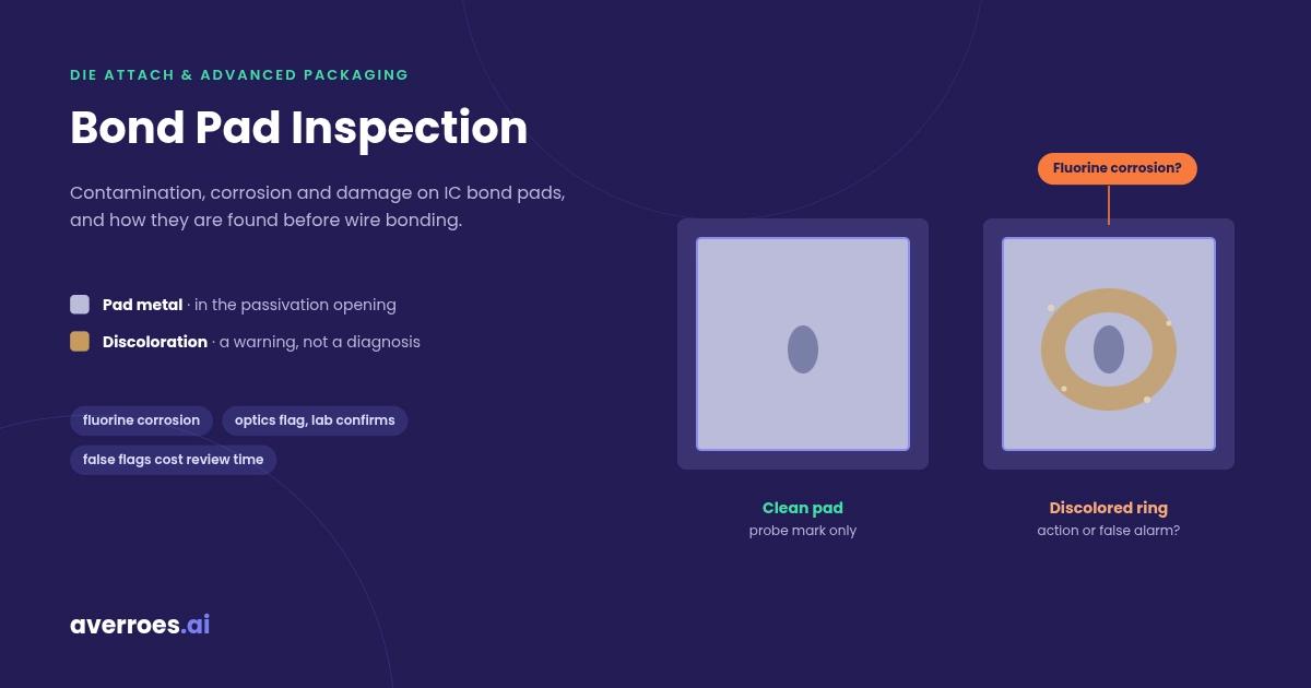
Probe mark inspection is the optical check of the marks probe needles leave on bond pads at wafer probe test, measuring their size, position and damage before the pads are wire bonded. Probing is not only a consumer of upstream defects: every touchdown creates a mark, and a bad mark is a defect of its own.
PMI matters because probe damage on the pad is a primary cause of wire bond failure, as EDN’s analysis of probe mark inspection put it. The inspection measures several things:
Mark size, including scrub length and width.
Location within the pad, and how close the mark comes to the pad edge.
Orientation relative to the pad center, and how that orientation trends across the wafer.
Failure signs such as excessive marking, punch-through to the layers below, and passivation not fully cleared from the pad.
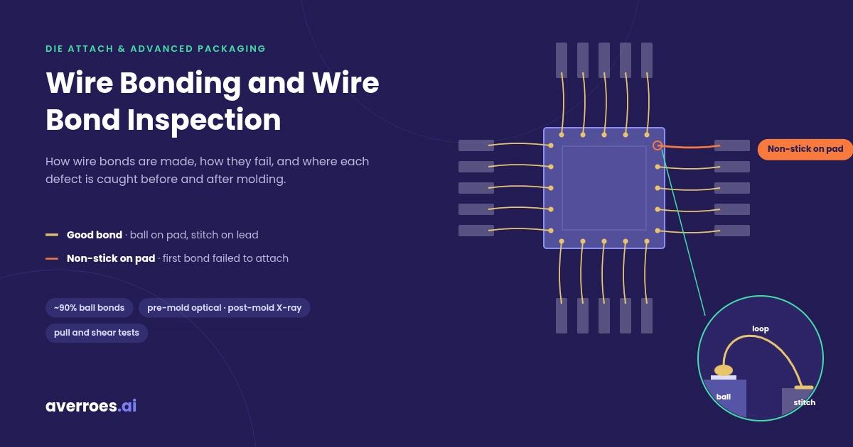
Pad damage shows up later as weaker bonds. A 2008 Southwest Test Workshop paper linked probe damage to lower ball shear and wire pull strength, and to more non-stick-on-pad and lifted ball bond failures. A study qualifying copper wire bonding set probe mark area at no more than 30% of the pad for a 35 ± 2 µm ball bond, and probe depth at no more than 80% of the original aluminum pad thickness. A separate IMAPS study on thin aluminum pads found that probe mark depth, not area, is the most adverse factor for bond reliability, so an inspection that measures area alone can pass a mark that is too deep.
Probe marks are small. A 2023 Chip Scale Review article described a 20 µm probe leaving a mark of about 16 × 12 µm, and showed probers that combine geometric algorithms with AI to detect the mark and correct probing offset automatically. Pad damage also feeds the reliability picture covered in semiconductor reliability testing.
The takeaway: a probe mark has to be judged by depth and position, not just by whether it is there.
Where AI Fits in Wafer Probe Test and Correlation
AI classification makes visual-electrical correlation more trustworthy by sorting inline detections into real defect classes and nuisance before they are overlaid on probe results. The correlation math does not change. What changes is the input: fewer falsely attributed defects, and kill ratios computed per real class instead of per raw detection.
AI does three jobs on the defect side of correlation:
Classify inline defects so each kill ratio is computed for a real defect class, with nuisance removed before overlay.
Monitor kill-ratio inputs over time, trending each defect class by layer, tool and lot so a rising killer class is visible before it shows up at probe test.
Read pattern signatures on defect maps and bin maps, so a spatial signature on one can be checked against the other.
Averroes.ai runs AI defect classification as an overlay on the inline inspection tools a fab already owns, including automated optical inspection for wafers. It trains models from 20 to 40 labeled images per defect class, with no code, and deploys on premise so wafer data stays inside the fab. Defect monitoring then trends the classified defects by layer, tool and lot, which is the data a kill-ratio pareto is built from. Averroes is not a prober or tester: it works on the inspection images and maps those tools produce.
Nuisance Defects Skewing Your Kill Ratios?
Test AI defect classification on your own inline defect data
Frequently Asked Questions
What is the difference between wafer sort and final test?
Wafer sort tests every die electrically while it is still on the wafer, before dicing and packaging. Final test checks the finished packaged parts. Probe contact limits some measurements at wafer sort, so final test can be more extensive. Sort keeps failing dies out of assembly, and final test confirms the packaged parts that passed.
What is a wafer acceptance test (WAT)?
A wafer acceptance test is a parametric test of dedicated structures in the scribe lines between dies, used to confirm that the process ran within its limits. It does not test the product dies, which is the job of wafer probe test. WAT probing can still leave marks that affect later steps.
What is a circuit probe (CP) test?
A circuit probe test is another name for wafer probe test: the electrical test of each die on a finished wafer using a prober, a probe card and a tester. Electronic die sort, electrical wafer sort and wafer final test are other common names for the same step.
What is a probe card?
A probe card is the fixture that carries the needles or probes used in wafer probe test, arranged in the exact pattern of a die’s bond pads. The prober presses the wafer against it so each probe contacts its pad, and the tester sends and reads signals through it.
What is kill ratio in semiconductor manufacturing?
Kill ratio is the probability that a defect of a given size, in a given layer, kills the die it lands on. It is calculated by overlaying inline defect maps on wafer probe results and dividing the number of failing dies with that defect by the total number of those defects found.
What is a wafer bin map?
A wafer bin map is a wafer-shaped grid with one cell per die, colored by the bin code each die received at wafer probe test. Pass bins mark good dies, and fail bins record which test a die failed. Spatial patterns on the map point engineers toward the process steps behind the failures.






A wafer probe test, also called wafer sort or circuit probe, is the electrical test of every die on a finished wafer before it is diced. A prober aligns the wafer, a probe card touches each die’s pads, and a tester runs parametric and functional tests. Each die gets a bin code, and the result is a wafer bin map. Overlaying that bin map on inline defect maps shows which visual defects actually kill dies.
Wafer probe test is Stage 05 of the semiconductor manufacturing process, between front-end fabrication and assembly. This guide from Averroes.ai, an AI visual inspection platform for manufacturers, covers how the test runs, how to read its bin maps, how probe marks are inspected, and how sort results are correlated with inline defect data.
Key Notes
What Is a Wafer Probe Test?
A wafer probe test, or wafer sort, is the electrical test of every die on a finished semiconductor wafer, run on a prober with a probe card and tester, to separate good dies from bad before assembly. It is the first time the chips on a wafer are tested as circuits rather than inspected as physical structures.
The step has several names. Wafer final test (WFT), electronic die sort (EDS) and circuit probe (CP) are among the most common, and probe card literature also calls it electrical wafer sort (EWS). All of them mean the same thing. One term needs separating: wafer sort is an electrical test, not a wafer sorter, which is a handling tool that moves wafers between carriers without testing them.
Wafer probe test sits in the wafer probe and electrical test stage of the hub, after the last front-end layer and before dicing. Dies that fail are excluded from assembly, so packaging cost is spent only on parts that passed.
Wafer Probe Test vs Wafer Acceptance Test
Wafer acceptance test (WAT) is a parametric test of dedicated structures in the scribe lines between dies, used to confirm the process ran within limits. Wafer probe test checks the product dies themselves. The two can interact: an IEEE case study traced a failure seen at wafer sort back to inline E-test probing on scribe-line structures, so even the test structures’ probe marks can become a defect source.
Wafer Probe Test vs Final Test
Final test checks packaged parts; wafer probe test checks dies while they are still on the wafer. Probe contact limits what can be measured, so the tests at wafer sort are not always as extensive as those at final test. Sort screens out the dies that should not be packaged, and final test confirms the parts that were.
How a Wafer Probe Test Works
A wafer probe test brings each die into contact with a probe card, runs a test program through an automatic tester, and records a pass or fail bin for every die. The prober handles the wafer, the probe card makes contact, and the tester runs the measurements.
A wafer probe test runs in 5 steps:
A probe card is the fixture that carries the needles or probes in the exact pattern of a die’s pads. The wafer prober is the machine that holds, aligns and steps the wafer under it. Both are deep topics on their own; this guide stays on what the test produces.
The takeaway: every die leaves wafer probe test with two records, a bin code and a probe mark.
How to Read a Wafer Bin Map
A wafer bin map is a wafer-shaped grid with one cell per die, colored by the bin code the die received at wafer probe test. Pass bins show good dies. Fail bins separate the failures by test, for example opens, shorts, leakage or speed, so the map shows both where dies failed and how.
Bin maps form spatial patterns, such as edge rings, center clusters and scratch lines, much as inline defect maps do. The pattern families and their usual causes are covered in wafer defect map analysis. A bin map shows electrical outcome, not physical cause. An edge ring of leakage fails says where yield was lost, but not which layer or tool caused it. That answer needs the inline data.
Bin maps and defect maps share one property that makes the next step possible: both use die coordinates referenced to the same notch. A defect at die (12, 7) on an inspection map and a fail at die (12, 7) on the bin map are the same die.
Correlating Visual Defect Maps With Electrical Test Results
Visual-electrical correlation overlays inline defect maps on the wafer probe bin map, die by die, to measure which defect classes actually cause electrical fails. Inline wafer inspection finds physical defects after each layer; wafer probe test finds electrical fails at the end. Correlation measures which of the first cause the second.
What each defect-to-bin overlay outcome means
The third row is the honest limit of correlation. Some electrical fails have no visible defect at any optical inspection step: buried shorts, parametric drift or defects below the inspected size. E-beam inspection with voltage contrast can find some of these inline, because it sees electrical behavior that optics cannot.
Kill Ratio in Semiconductor Yield
Kill ratio is the probability that a defect of a given size, in a given layer, kills the die it lands on. A 1999 SPIE paper by Lorenzo and colleagues defined it this way and computed it by correlating inline inspection data with test results. In words, a defect class’s kill ratio is the number of dies with that defect that failed, divided by the total number of those defects found.
A simpler method correlates defect counts per wafer with wafer yield. Kill ratio is sharper because it works per die and per class. Once each class has a kill ratio, defect counts become a yield loss pareto: the list of defect classes ranked by the dies they cost. That pareto is what decides which defect to chase first. The defect classes themselves follow the structure laid out in the wafer defect classification taxonomy.
Defect-Limited Yield
Defect-limited yield is the yield a wafer would have if defects were the only cause of failure, estimated from defect densities and kill ratios layer by layer. It shows which layer costs the most dies. A layer with few defects but a high kill ratio can cost more yield than a layer with many harmless ones. Random particles set the baseline; particle contamination inspection covers how that baseline is tracked.
Why Correlation Goes Wrong
Correlation is only as accurate as the defect data fed into it. A published paper on bitmap-to-defect correlation warned that too wide an overlay tolerance or an overly sensitive inspection recipe adds falsely attributed defects: detections that land on a failing die by chance and get counted as its cause. Because inspection runs at many layers, a small error per layer adds up, and the yield loss pareto ends up ranking the wrong defect classes.
Two other limits apply. Inline inspection is sampled, so not every wafer that reaches probe test has full defect data. And nuisance detections, signals that are not real defects, inflate the “defect but passed” row and dilute the kill ratio of the classes that matter. Once a killer class is identified, automated root cause analysis traces it to the tool and step behind it.
The takeaway: kill ratio is only as clean as the defect classes that feed it.
Probe Mark Inspection (PMI)
Probe mark inspection is the optical check of the marks probe needles leave on bond pads at wafer probe test, measuring their size, position and damage before the pads are wire bonded. Probing is not only a consumer of upstream defects: every touchdown creates a mark, and a bad mark is a defect of its own.
PMI matters because probe damage on the pad is a primary cause of wire bond failure, as EDN’s analysis of probe mark inspection put it. The inspection measures several things:
Pad damage shows up later as weaker bonds. A 2008 Southwest Test Workshop paper linked probe damage to lower ball shear and wire pull strength, and to more non-stick-on-pad and lifted ball bond failures. A study qualifying copper wire bonding set probe mark area at no more than 30% of the pad for a 35 ± 2 µm ball bond, and probe depth at no more than 80% of the original aluminum pad thickness. A separate IMAPS study on thin aluminum pads found that probe mark depth, not area, is the most adverse factor for bond reliability, so an inspection that measures area alone can pass a mark that is too deep.
Probe marks are small. A 2023 Chip Scale Review article described a 20 µm probe leaving a mark of about 16 × 12 µm, and showed probers that combine geometric algorithms with AI to detect the mark and correct probing offset automatically. Pad damage also feeds the reliability picture covered in semiconductor reliability testing.
The takeaway: a probe mark has to be judged by depth and position, not just by whether it is there.
Where AI Fits in Wafer Probe Test and Correlation
AI classification makes visual-electrical correlation more trustworthy by sorting inline detections into real defect classes and nuisance before they are overlaid on probe results. The correlation math does not change. What changes is the input: fewer falsely attributed defects, and kill ratios computed per real class instead of per raw detection.
AI does three jobs on the defect side of correlation:
Averroes.ai runs AI defect classification as an overlay on the inline inspection tools a fab already owns, including automated optical inspection for wafers. It trains models from 20 to 40 labeled images per defect class, with no code, and deploys on premise so wafer data stays inside the fab. Defect monitoring then trends the classified defects by layer, tool and lot, which is the data a kill-ratio pareto is built from. Averroes is not a prober or tester: it works on the inspection images and maps those tools produce.
Nuisance Defects Skewing Your Kill Ratios?
Test AI defect classification on your own inline defect data
Frequently Asked Questions
What is the difference between wafer sort and final test?
Wafer sort tests every die electrically while it is still on the wafer, before dicing and packaging. Final test checks the finished packaged parts. Probe contact limits some measurements at wafer sort, so final test can be more extensive. Sort keeps failing dies out of assembly, and final test confirms the packaged parts that passed.
What is a wafer acceptance test (WAT)?
A wafer acceptance test is a parametric test of dedicated structures in the scribe lines between dies, used to confirm that the process ran within its limits. It does not test the product dies, which is the job of wafer probe test. WAT probing can still leave marks that affect later steps.
What is a circuit probe (CP) test?
A circuit probe test is another name for wafer probe test: the electrical test of each die on a finished wafer using a prober, a probe card and a tester. Electronic die sort, electrical wafer sort and wafer final test are other common names for the same step.
What is a probe card?
A probe card is the fixture that carries the needles or probes used in wafer probe test, arranged in the exact pattern of a die’s bond pads. The prober presses the wafer against it so each probe contacts its pad, and the tester sends and reads signals through it.
What is kill ratio in semiconductor manufacturing?
Kill ratio is the probability that a defect of a given size, in a given layer, kills the die it lands on. It is calculated by overlaying inline defect maps on wafer probe results and dividing the number of failing dies with that defect by the total number of those defects found.
What is a wafer bin map?
A wafer bin map is a wafer-shaped grid with one cell per die, colored by the bin code each die received at wafer probe test. Pass bins mark good dies, and fail bins record which test a die failed. Spatial patterns on the map point engineers toward the process steps behind the failures.